Workflow Example#
Here we illustrate a complete workflow example including the following steps:
Data loading
Converting the data to CF format
Preprocessing the data
Running a diagnostic
Visualizing the results
Imports#
[1]:
from pathlib import Path

import xarray as xr
from datatree import DataTree

import valenspy as vp #The Valenspy package
from valenspy.inputconverter_functions import _non_convertor
Input Convertors#
Input convertors are used to convert the data to CF format. There main component is a function that takes the file and returns the data CF convention. See input_convertors_functions.py for examples.
The Input convertor is a class that does the following:
Convert the data
Check if the converted data meets the CF convention
…
[2]:
#Import Converter - This input converter will not do anything to the data.
ic = vp.InputConverter(_non_convertor)
Loading datasets#
Load the data and convert to CF format if necessary.
In this illustration we will load EOBS data, CMIP6 historical and future data
[3]:
#Observational dataset
EOBS_data_dir = Path("/dodrio/scratch/projects/2022_200/project_input/External/observations/EOBS/0.1deg/")

EOBS_obs_files = list(EOBS_data_dir.glob("*tg*mean*.nc")) #Select all the netCDF files in the directory
EOBS_obs_files = ic.convert_input(EOBS_obs_files) #Convert the input to the correct format

EOBS_ds = xr.open_mfdataset(EOBS_obs_files, combine='by_coords', chunks='auto')

#THIS SHOULD ALL BE IN THE INPUT CONVERTER FOR THE DATASET
EOBS_ds = EOBS_ds.rename_vars({"tg": "tas"})
EOBS_ds = EOBS_ds.rename({"latitude": "lat", "longitude": "lon"})
#Convert from Celsius to Kelvin
EOBS_ds["tas"] = EOBS_ds["tas"] + 273.15

#Select a small region covering Belgium for testing
EOBS_ds = EOBS_ds.sel(time=slice("1953-01-01", "1954-12-31"))
EOBS_ds = EOBS_ds.sel(lat=slice(49, 51), lon=slice(3, 5))

EOBS_ds
[3]:
<xarray.Dataset> Size: 1MB
Dimensions:  (lat: 20, lon: 20, time: 730)
Coordinates:
  * lat      (lat) float64 160B 49.05 49.15 49.25 49.35 ... 50.75 50.85 50.95
  * lon      (lon) float64 160B 3.05 3.15 3.25 3.35 3.45 ... 4.65 4.75 4.85 4.95
  * time     (time) datetime64[ns] 6kB 1953-01-01 1953-01-02 ... 1954-12-31
Data variables:
    tas      (time, lat, lon) float32 1MB dask.array<chunksize=(26, 20, 20), meta=np.ndarray>
Attributes:
    E-OBS_version:  29.0e
    Conventions:    CF-1.4
    References:     http://surfobs.climate.copernicus.eu/dataaccess/access_eo...
    history:        Fri Mar 22 09:55:59 2024: ncks --no-abc -d time,0,27027 /...
NCO: netCDF Operators version 5.1.4 (Homepage = http://nco.sf....- lat: 20
- lon: 20
- time: 730
- lat(lat)float6449.05 49.15 49.25 ... 50.85 50.95
- units :
- degrees_north
- long_name :
- Latitude values
- axis :
- Y
- standard_name :
- latitude
array([49.049861, 49.149861, 49.249861, 49.349861, 49.449861, 49.549861, 49.649861, 49.749861, 49.849861, 49.949861, 50.049861, 50.149861, 50.249861, 50.349861, 50.449861, 50.549861, 50.649861, 50.749861, 50.849861, 50.949861]) - lon(lon)float643.05 3.15 3.25 ... 4.75 4.85 4.95
- units :
- degrees_east
- long_name :
- Longitude values
- axis :
- X
- standard_name :
- longitude
array([3.04986, 3.14986, 3.24986, 3.34986, 3.44986, 3.54986, 3.64986, 3.74986, 3.84986, 3.94986, 4.04986, 4.14986, 4.24986, 4.34986, 4.44986, 4.54986, 4.64986, 4.74986, 4.84986, 4.94986]) - time(time)datetime64[ns]1953-01-01 ... 1954-12-31
- long_name :
- Time in days
- standard_name :
- time
- cell_methods :
- time: mean
array(['1953-01-01T00:00:00.000000000', '1953-01-02T00:00:00.000000000',
       '1953-01-03T00:00:00.000000000', ..., '1954-12-29T00:00:00.000000000',
       '1954-12-30T00:00:00.000000000', '1954-12-31T00:00:00.000000000'],
      dtype='datetime64[ns]')
- tas(time, lat, lon)float32dask.array<chunksize=(26, 20, 20), meta=np.ndarray>
Array Chunk Bytes 1.11 MiB 159.38 kiB Shape (730, 20, 20) (102, 20, 20) Dask graph 8 chunks in 5 graph layers Data type float32 numpy.ndarray
- latPandasIndex
PandasIndex(Index([ 49.04986053396604, 49.14986053364869, 49.24986053333134, 49.349860533014, 49.44986053269666, 49.54986053237931, 49.649860532061965, 49.74986053174462, 49.84986053142728, 49.949860531109934, 50.049860530792586, 50.149860530475245, 50.2498605301579, 50.349860529840555, 50.44986052952321, 50.549860529205866, 50.649860528888524, 50.749860528571176, 50.84986052825383, 50.94986052793648], dtype='float64', name='lat')) - lonPandasIndex
PandasIndex(Index([ 3.049860378785798, 3.149860378385746, 3.2498603779856943, 3.3498603775856424, 3.4498603771855905, 3.5498603767855386, 3.6498603763854867, 3.7498603759854348, 3.849860375585383, 3.949860375185331, 4.049860374785279, 4.149860374385227, 4.249860373985175, 4.349860373585123, 4.449860373185071, 4.5498603727850195, 4.649860372384968, 4.749860371984916, 4.849860371584864, 4.949860371184812], dtype='float64', name='lon')) - timePandasIndex
PandasIndex(DatetimeIndex(['1953-01-01', '1953-01-02', '1953-01-03', '1953-01-04',
               '1953-01-05', '1953-01-06', '1953-01-07', '1953-01-08',
               '1953-01-09', '1953-01-10',
               ...
               '1954-12-22', '1954-12-23', '1954-12-24', '1954-12-25',
               '1954-12-26', '1954-12-27', '1954-12-28', '1954-12-29',
               '1954-12-30', '1954-12-31'],
              dtype='datetime64[ns]', name='time', length=730, freq=None))
- E-OBS_version :
- 29.0e
- Conventions :
- CF-1.4
- References :
- http://surfobs.climate.copernicus.eu/dataaccess/access_eobs.php
- history :
- Fri Mar 22 09:55:59 2024: ncks --no-abc -d time,0,27027 /nobackup_1/users/besselaa/Data/Gridding/EOBSv29.0e/Grid_0.1deg/tg//tg_ensmean_master_rectime.nc /nobackup_1/users/besselaa/Data/Gridding/EOBSv29.0e/Grid_0.1deg/tg//tg_ens_mean_0.1deg_reg_v29.0e.nc Fri Mar 22 09:50:30 2024: ncks --no-abc --mk_rec_dmn time /nobackup_1/users/besselaa/Data/Gridding/EOBSv29.0e/Grid_0.1deg/tg//tg_ensmean_master.nc /nobackup_1/users/besselaa/Data/Gridding/EOBSv29.0e/Grid_0.1deg/tg//tg_ensmean_master_rectime.nc Fri Mar 22 09:32:14 2024: ncks -O -d time,0,27027 /nobackup_1/users/besselaa/Data/Gridding/EOBSv29.0e/Grid_0.1deg/tg/tg_ensmean_master_untilJan2024.nc /nobackup_1/users/besselaa/Data/Gridding/EOBSv29.0e/Grid_0.1deg/tg/tg_ensmean_master.nc
- NCO :
- netCDF Operators version 5.1.4 (Homepage = http://nco.sf.net, Code = http://github.com/nco/nco)
[4]:
#CMIP6 dataset
#Now make an ensemble member object
EC_Earth3_dir = Path("/dodrio/scratch/projects/2022_200/project_output/RMIB-UGent/vsc46032_kobe/ValEnsPy/tests/data")
EC_Earth3_hist_files = list(EC_Earth3_dir.glob("*historical*.nc")) #Select all the netCDF files in the directory
EC_Earth3_hist_files = ic.convert_input(EC_Earth3_hist_files) #Convert the input to the correct format
EC_Earth3_ds = xr.open_mfdataset(EC_Earth3_hist_files, combine='by_coords', chunks='auto')
EC_Earth3_ds
[4]:
<xarray.Dataset> Size: 13MB
Dimensions:    (time: 24, bnds: 2, lat: 256, lon: 512)
Coordinates:
  * time       (time) datetime64[ns] 192B 1953-01-16T12:00:00 ... 1954-12-16T...
  * lat        (lat) float64 2kB -89.46 -88.77 -88.07 ... 88.07 88.77 89.46
  * lon        (lon) float64 4kB 0.0 0.7031 1.406 2.109 ... 357.9 358.6 359.3
    height     float64 8B 2.0
Dimensions without coordinates: bnds
Data variables:
    time_bnds  (time, bnds) datetime64[ns] 384B dask.array<chunksize=(12, 2), meta=np.ndarray>
    lat_bnds   (time, lat, bnds) float64 98kB dask.array<chunksize=(12, 256, 2), meta=np.ndarray>
    lon_bnds   (time, lon, bnds) float64 197kB dask.array<chunksize=(12, 512, 2), meta=np.ndarray>
    tas        (time, lat, lon) float32 13MB dask.array<chunksize=(12, 256, 512), meta=np.ndarray>
Attributes: (12/46)
    Conventions:                        CF-1.7 CMIP-6.2
    activity_id:                        CMIP
    branch_method:                      standard
    branch_time_in_child:               0.0
    branch_time_in_parent:              29219.0
    contact:                            cmip6-data@ec-earth.org
    ...                                 ...
    variant_label:                      r1i1p1f1
    license:                            CMIP6 model data produced by EC-Earth...
    cmor_version:                       3.4.0
    tracking_id:                        hdl:21.14100/18af2970-6a17-45fe-b629-...
    history:                            2019-06-06T07:27:13Z ; CMOR rewrote d...
latest_applied_cmor_fixer_version: v3.0- time: 24
- bnds: 2
- lat: 256
- lon: 512
- time(time)datetime64[ns]1953-01-16T12:00:00 ... 1954-12-...
- bounds :
- time_bnds
- axis :
- T
- long_name :
- time
- standard_name :
- time
array(['1953-01-16T12:00:00.000000000', '1953-02-15T00:00:00.000000000', '1953-03-16T12:00:00.000000000', '1953-04-16T00:00:00.000000000', '1953-05-16T12:00:00.000000000', '1953-06-16T00:00:00.000000000', '1953-07-16T12:00:00.000000000', '1953-08-16T12:00:00.000000000', '1953-09-16T00:00:00.000000000', '1953-10-16T12:00:00.000000000', '1953-11-16T00:00:00.000000000', '1953-12-16T12:00:00.000000000', '1954-01-16T12:00:00.000000000', '1954-02-15T00:00:00.000000000', '1954-03-16T12:00:00.000000000', '1954-04-16T00:00:00.000000000', '1954-05-16T12:00:00.000000000', '1954-06-16T00:00:00.000000000', '1954-07-16T12:00:00.000000000', '1954-08-16T12:00:00.000000000', '1954-09-16T00:00:00.000000000', '1954-10-16T12:00:00.000000000', '1954-11-16T00:00:00.000000000', '1954-12-16T12:00:00.000000000'], dtype='datetime64[ns]') - lat(lat)float64-89.46 -88.77 ... 88.77 89.46
- bounds :
- lat_bnds
- units :
- degrees_north
- axis :
- Y
- long_name :
- Latitude
- standard_name :
- latitude
array([-89.462822, -88.766951, -88.066972, ..., 88.066972, 88.766951, 89.462822]) - lon(lon)float640.0 0.7031 1.406 ... 358.6 359.3
- bounds :
- lon_bnds
- units :
- degrees_east
- axis :
- X
- long_name :
- Longitude
- standard_name :
- longitude
array([ 0. , 0.703125, 1.40625 , ..., 357.890625, 358.59375 , 359.296875]) - height()float642.0
- units :
- m
- axis :
- Z
- positive :
- up
- long_name :
- height
- standard_name :
- height
array(2.)
- time_bnds(time, bnds)datetime64[ns]dask.array<chunksize=(12, 2), meta=np.ndarray>
Array Chunk Bytes 384 B 192 B Shape (24, 2) (12, 2) Dask graph 2 chunks in 5 graph layers Data type datetime64[ns] numpy.ndarray - lat_bnds(time, lat, bnds)float64dask.array<chunksize=(12, 256, 2), meta=np.ndarray>
Array Chunk Bytes 96.00 kiB 48.00 kiB Shape (24, 256, 2) (12, 256, 2) Dask graph 2 chunks in 7 graph layers Data type float64 numpy.ndarray - lon_bnds(time, lon, bnds)float64dask.array<chunksize=(12, 512, 2), meta=np.ndarray>
Array Chunk Bytes 192.00 kiB 96.00 kiB Shape (24, 512, 2) (12, 512, 2) Dask graph 2 chunks in 7 graph layers Data type float64 numpy.ndarray - tas(time, lat, lon)float32dask.array<chunksize=(12, 256, 512), meta=np.ndarray>
- standard_name :
- air_temperature
- long_name :
- Near-Surface Air Temperature
- comment :
- near-surface (usually, 2 meter) air temperature
- units :
- K
- cell_methods :
- area: time: mean
- cell_measures :
- area: areacella
- history :
- 2019-06-06T07:27:13Z altered by CMOR: Treated scalar dimension: 'height'. 2019-06-06T07:27:13Z altered by CMOR: Reordered dimensions, original order: lat lon time.
Array Chunk Bytes 12.00 MiB 6.00 MiB Shape (24, 256, 512) (12, 256, 512) Dask graph 2 chunks in 5 graph layers Data type float32 numpy.ndarray
- timePandasIndex
PandasIndex(DatetimeIndex(['1953-01-16 12:00:00', '1953-02-15 00:00:00', '1953-03-16 12:00:00', '1953-04-16 00:00:00', '1953-05-16 12:00:00', '1953-06-16 00:00:00', '1953-07-16 12:00:00', '1953-08-16 12:00:00', '1953-09-16 00:00:00', '1953-10-16 12:00:00', '1953-11-16 00:00:00', '1953-12-16 12:00:00', '1954-01-16 12:00:00', '1954-02-15 00:00:00', '1954-03-16 12:00:00', '1954-04-16 00:00:00', '1954-05-16 12:00:00', '1954-06-16 00:00:00', '1954-07-16 12:00:00', '1954-08-16 12:00:00', '1954-09-16 00:00:00', '1954-10-16 12:00:00', '1954-11-16 00:00:00', '1954-12-16 12:00:00'], dtype='datetime64[ns]', name='time', freq=None)) - latPandasIndex
PandasIndex(Index([-89.4628215685774, -88.7669513528422, -88.0669716474306, -87.366063433082, -86.6648030134408, -85.9633721608804, -85.2618460607126, -84.5602613830534, -83.8586381286076, -83.1569881285417, ... 83.1569881285417, 83.8586381286076, 84.5602613830534, 85.2618460607126, 85.9633721608804, 86.6648030134408, 87.366063433082, 88.0669716474306, 88.7669513528422, 89.4628215685774], dtype='float64', name='lat', length=256)) - lonPandasIndex
PandasIndex(Index([       0.0,   0.703125,    1.40625,   2.109375,     2.8125,   3.515625,
          4.21875,   4.921875,      5.625,   6.328125,
       ...
        352.96875, 353.671875,    354.375, 355.078125,  355.78125, 356.484375,
         357.1875, 357.890625,  358.59375, 359.296875],
      dtype='float64', name='lon', length=512))
- Conventions :
- CF-1.7 CMIP-6.2
- activity_id :
- CMIP
- branch_method :
- standard
- branch_time_in_child :
- 0.0
- branch_time_in_parent :
- 29219.0
- contact :
- cmip6-data@ec-earth.org
- creation_date :
- 2019-06-06T07:27:13Z
- data_specs_version :
- 01.00.30
- experiment :
- all-forcing simulation of the recent past
- experiment_id :
- historical
- external_variables :
- areacella
- forcing_index :
- 1
- frequency :
- mon
- further_info_url :
- https://furtherinfo.es-doc.org/CMIP6.EC-Earth-Consortium.EC-Earth3-Veg.historical.none.r1i1p1f1
- grid :
- T255L91-ORCA1L75
- grid_label :
- gr
- initialization_index :
- 1
- institution :
- AEMET, Spain; BSC, Spain; CNR-ISAC, Italy; DMI, Denmark; ENEA, Italy; FMI, Finland; Geomar, Germany; ICHEC, Ireland; ICTP, Italy; IDL, Portugal; IMAU, The Netherlands; IPMA, Portugal; KIT, Karlsruhe, Germany; KNMI, The Netherlands; Lund University, Sweden; Met Eireann, Ireland; NLeSC, The Netherlands; NTNU, Norway; Oxford University, UK; surfSARA, The Netherlands; SMHI, Sweden; Stockholm University, Sweden; Unite ASTR, Belgium; University College Dublin, Ireland; University of Bergen, Norway; University of Copenhagen, Denmark; University of Helsinki, Finland; University of Santiago de Compostela, Spain; Uppsala University, Sweden; Utrecht University, The Netherlands; Vrije Universiteit Amsterdam, the Netherlands; Wageningen University, The Netherlands. Mailing address: EC-Earth consortium, Rossby Center, Swedish Meteorological and Hydrological Institute/SMHI, SE-601 76 Norrkoping, Sweden
- institution_id :
- EC-Earth-Consortium
- mip_era :
- CMIP6
- nominal_resolution :
- 100 km
- parent_activity_id :
- CMIP
- parent_experiment_id :
- piControl
- parent_mip_era :
- CMIP6
- parent_source_id :
- EC-Earth3-Veg
- parent_time_units :
- days since 1850-01-01
- parent_variant_label :
- r1i1p1f1
- physics_index :
- 1
- product :
- model-output
- realization_index :
- 1
- realm :
- atmos
- source :
- EC-Earth3-Veg (2019): aerosol: none atmos: IFS cy36r4 (TL255, linearly reduced Gaussian grid equivalent to 512 x 256 longitude/latitude; 91 levels; top level 0.01 hPa) atmosChem: none land: HTESSEL (land surface scheme built in IFS) and LPJ-GUESS v4 landIce: none ocean: NEMO3.6 (ORCA1 tripolar primarily 1 degree with meridional refinement down to 1/3 degree in the tropics; 362 x 292 longitude/latitude; 75 levels; top grid cell 0-1 m) ocnBgchem: none seaIce: LIM3
- source_id :
- EC-Earth3-Veg
- source_type :
- AOGCM
- sub_experiment :
- none
- sub_experiment_id :
- none
- table_id :
- Amon
- table_info :
- Creation Date:(09 May 2019) MD5:cde930676e68ac6780d5e4c62d3898f6
- title :
- EC-Earth3-Veg output prepared for CMIP6
- variable_id :
- tas
- variant_label :
- r1i1p1f1
- license :
- CMIP6 model data produced by EC-Earth-Consortium is licensed under a Creative Commons Attribution-ShareAlike 4.0 International License (https://creativecommons.org/licenses). Consult https://pcmdi.llnl.gov/CMIP6/TermsOfUse for terms of use governing CMIP6 output, including citation requirements and proper acknowledgment. Further information about this data, including some limitations, can be found via the further_info_url (recorded as a global attribute in this file) and at http://www.ec-earth.org. The data producers and data providers make no warranty, either express or implied, including, but not limited to, warranties of merchantability and fitness for a particular purpose. All liabilities arising from the supply of the information (including any liability arising in negligence) are excluded to the fullest extent permitted by law.
- cmor_version :
- 3.4.0
- tracking_id :
- hdl:21.14100/18af2970-6a17-45fe-b629-86d0fc18a6c1
- history :
- 2019-06-06T07:27:13Z ; CMOR rewrote data to be consistent with CMIP6, CF-1.7 CMIP-6.2 and CF standards.; processed by ece2cmor vv1.1.0, git rev. 032f6287076b212e5c49922af94a0ddecb191a16 The cmor-fixer version v2.1 script has been applied.The cmor-fixer version v3.0 script has been applied.
- latest_applied_cmor_fixer_version :
- v3.0
[5]:
#Now make an "future" ensemble member object
EC_Earth3_ssp_files = list(EC_Earth3_dir.glob("*ssp245*.nc")) #Select all the netCDF files in the directory
EC_Earth3_ssp_files = ic.convert_input(EC_Earth3_ssp_files) #Convert the input to the correct format
EC_Earth3_ssp_ds = xr.open_mfdataset(EC_Earth3_ssp_files, combine='by_coords', chunks='auto')
EC_Earth3_ssp_ds
[5]:
<xarray.Dataset> Size: 13MB
Dimensions:    (time: 24, bnds: 2, lat: 256, lon: 512)
Coordinates:
  * time       (time) datetime64[ns] 192B 2015-01-16T12:00:00 ... 2016-12-16T...
  * lat        (lat) float64 2kB -89.46 -88.77 -88.07 ... 88.07 88.77 89.46
  * lon        (lon) float64 4kB 0.0 0.7031 1.406 2.109 ... 357.9 358.6 359.3
    height     float64 8B 2.0
Dimensions without coordinates: bnds
Data variables:
    time_bnds  (time, bnds) datetime64[ns] 384B dask.array<chunksize=(12, 2), meta=np.ndarray>
    lat_bnds   (time, lat, bnds) float64 98kB dask.array<chunksize=(12, 256, 2), meta=np.ndarray>
    lon_bnds   (time, lon, bnds) float64 197kB dask.array<chunksize=(12, 512, 2), meta=np.ndarray>
    tas        (time, lat, lon) float32 13MB dask.array<chunksize=(12, 256, 512), meta=np.ndarray>
Attributes: (12/45)
    Conventions:            CF-1.7 CMIP-6.2
    activity_id:            ScenarioMIP
    branch_method:          standard
    branch_time_in_child:   60265.0
    branch_time_in_parent:  60265.0
    contact:                cmip6-data@ec-earth.org
    ...                     ...
    variable_id:            tas
    variant_label:          r1i1p1f1
    license:                CMIP6 model data produced by EC-Earth-Consortium ...
    cmor_version:           3.4.0
    tracking_id:            hdl:21.14100/697b3a82-4ffc-49ce-b070-2ca86ce8a06f
history: 2019-06-29T08:25:09Z ; CMOR rewrote data to be co...- time: 24
- bnds: 2
- lat: 256
- lon: 512
- time(time)datetime64[ns]2015-01-16T12:00:00 ... 2016-12-...
- bounds :
- time_bnds
- axis :
- T
- long_name :
- time
- standard_name :
- time
array(['2015-01-16T12:00:00.000000000', '2015-02-15T00:00:00.000000000', '2015-03-16T12:00:00.000000000', '2015-04-16T00:00:00.000000000', '2015-05-16T12:00:00.000000000', '2015-06-16T00:00:00.000000000', '2015-07-16T12:00:00.000000000', '2015-08-16T12:00:00.000000000', '2015-09-16T00:00:00.000000000', '2015-10-16T12:00:00.000000000', '2015-11-16T00:00:00.000000000', '2015-12-16T12:00:00.000000000', '2016-01-16T12:00:00.000000000', '2016-02-15T12:00:00.000000000', '2016-03-16T12:00:00.000000000', '2016-04-16T00:00:00.000000000', '2016-05-16T12:00:00.000000000', '2016-06-16T00:00:00.000000000', '2016-07-16T12:00:00.000000000', '2016-08-16T12:00:00.000000000', '2016-09-16T00:00:00.000000000', '2016-10-16T12:00:00.000000000', '2016-11-16T00:00:00.000000000', '2016-12-16T12:00:00.000000000'], dtype='datetime64[ns]') - lat(lat)float64-89.46 -88.77 ... 88.77 89.46
- bounds :
- lat_bnds
- units :
- degrees_north
- axis :
- Y
- long_name :
- Latitude
- standard_name :
- latitude
array([-89.462822, -88.766951, -88.066972, ..., 88.066972, 88.766951, 89.462822]) - lon(lon)float640.0 0.7031 1.406 ... 358.6 359.3
- bounds :
- lon_bnds
- units :
- degrees_east
- axis :
- X
- long_name :
- Longitude
- standard_name :
- longitude
array([ 0. , 0.703125, 1.40625 , ..., 357.890625, 358.59375 , 359.296875]) - height()float642.0
- units :
- m
- axis :
- Z
- positive :
- up
- long_name :
- height
- standard_name :
- height
array(2.)
- time_bnds(time, bnds)datetime64[ns]dask.array<chunksize=(12, 2), meta=np.ndarray>
Array Chunk Bytes 384 B 192 B Shape (24, 2) (12, 2) Dask graph 2 chunks in 5 graph layers Data type datetime64[ns] numpy.ndarray - lat_bnds(time, lat, bnds)float64dask.array<chunksize=(12, 256, 2), meta=np.ndarray>
Array Chunk Bytes 96.00 kiB 48.00 kiB Shape (24, 256, 2) (12, 256, 2) Dask graph 2 chunks in 7 graph layers Data type float64 numpy.ndarray - lon_bnds(time, lon, bnds)float64dask.array<chunksize=(12, 512, 2), meta=np.ndarray>
Array Chunk Bytes 192.00 kiB 96.00 kiB Shape (24, 512, 2) (12, 512, 2) Dask graph 2 chunks in 7 graph layers Data type float64 numpy.ndarray - tas(time, lat, lon)float32dask.array<chunksize=(12, 256, 512), meta=np.ndarray>
- standard_name :
- air_temperature
- long_name :
- Near-Surface Air Temperature
- comment :
- near-surface (usually, 2 meter) air temperature
- units :
- K
- cell_methods :
- area: time: mean
- cell_measures :
- area: areacella
- history :
- 2019-06-29T08:25:09Z altered by CMOR: Treated scalar dimension: 'height'. 2019-06-29T08:25:09Z altered by CMOR: Reordered dimensions, original order: lat lon time.
Array Chunk Bytes 12.00 MiB 6.00 MiB Shape (24, 256, 512) (12, 256, 512) Dask graph 2 chunks in 5 graph layers Data type float32 numpy.ndarray
- timePandasIndex
PandasIndex(DatetimeIndex(['2015-01-16 12:00:00', '2015-02-15 00:00:00', '2015-03-16 12:00:00', '2015-04-16 00:00:00', '2015-05-16 12:00:00', '2015-06-16 00:00:00', '2015-07-16 12:00:00', '2015-08-16 12:00:00', '2015-09-16 00:00:00', '2015-10-16 12:00:00', '2015-11-16 00:00:00', '2015-12-16 12:00:00', '2016-01-16 12:00:00', '2016-02-15 12:00:00', '2016-03-16 12:00:00', '2016-04-16 00:00:00', '2016-05-16 12:00:00', '2016-06-16 00:00:00', '2016-07-16 12:00:00', '2016-08-16 12:00:00', '2016-09-16 00:00:00', '2016-10-16 12:00:00', '2016-11-16 00:00:00', '2016-12-16 12:00:00'], dtype='datetime64[ns]', name='time', freq=None)) - latPandasIndex
PandasIndex(Index([-89.4628215685774, -88.7669513528422, -88.0669716474306, -87.366063433082, -86.6648030134408, -85.9633721608804, -85.2618460607126, -84.5602613830534, -83.8586381286076, -83.1569881285417, ... 83.1569881285417, 83.8586381286076, 84.5602613830534, 85.2618460607126, 85.9633721608804, 86.6648030134408, 87.366063433082, 88.0669716474306, 88.7669513528422, 89.4628215685774], dtype='float64', name='lat', length=256)) - lonPandasIndex
PandasIndex(Index([       0.0,   0.703125,    1.40625,   2.109375,     2.8125,   3.515625,
          4.21875,   4.921875,      5.625,   6.328125,
       ...
        352.96875, 353.671875,    354.375, 355.078125,  355.78125, 356.484375,
         357.1875, 357.890625,  358.59375, 359.296875],
      dtype='float64', name='lon', length=512))
- Conventions :
- CF-1.7 CMIP-6.2
- activity_id :
- ScenarioMIP
- branch_method :
- standard
- branch_time_in_child :
- 60265.0
- branch_time_in_parent :
- 60265.0
- contact :
- cmip6-data@ec-earth.org
- creation_date :
- 2019-06-29T08:25:09Z
- data_specs_version :
- 01.00.30
- experiment :
- update of RCP4.5 based on SSP2
- experiment_id :
- ssp245
- external_variables :
- areacella
- forcing_index :
- 1
- frequency :
- mon
- further_info_url :
- https://furtherinfo.es-doc.org/CMIP6.EC-Earth-Consortium.EC-Earth3-Veg.ssp245.none.r1i1p1f1
- grid :
- T255L91-ORCA1L75
- grid_label :
- gr
- initialization_index :
- 1
- institution :
- AEMET, Spain; BSC, Spain; CNR-ISAC, Italy; DMI, Denmark; ENEA, Italy; FMI, Finland; Geomar, Germany; ICHEC, Ireland; ICTP, Italy; IDL, Portugal; IMAU, The Netherlands; IPMA, Portugal; KIT, Karlsruhe, Germany; KNMI, The Netherlands; Lund University, Sweden; Met Eireann, Ireland; NLeSC, The Netherlands; NTNU, Norway; Oxford University, UK; surfSARA, The Netherlands; SMHI, Sweden; Stockholm University, Sweden; Unite ASTR, Belgium; University College Dublin, Ireland; University of Bergen, Norway; University of Copenhagen, Denmark; University of Helsinki, Finland; University of Santiago de Compostela, Spain; Uppsala University, Sweden; Utrecht University, The Netherlands; Vrije Universiteit Amsterdam, the Netherlands; Wageningen University, The Netherlands. Mailing address: EC-Earth consortium, Rossby Center, Swedish Meteorological and Hydrological Institute/SMHI, SE-601 76 Norrkoping, Sweden
- institution_id :
- EC-Earth-Consortium
- mip_era :
- CMIP6
- nominal_resolution :
- 100 km
- parent_activity_id :
- CMIP
- parent_experiment_id :
- historical
- parent_mip_era :
- CMIP6
- parent_source_id :
- EC-Earth3-Veg
- parent_time_units :
- days since 1850-01-01
- parent_variant_label :
- r1i1p1f1
- physics_index :
- 1
- product :
- model-output
- realization_index :
- 1
- realm :
- atmos
- source :
- EC-Earth3-Veg (2019): aerosol: none atmos: IFS cy36r4 (TL255, linearly reduced Gaussian grid equivalent to 512 x 256 longitude/latitude; 91 levels; top level 0.01 hPa) atmosChem: none land: HTESSEL (land surface scheme built in IFS) and LPJ-GUESS v4 landIce: none ocean: NEMO3.6 (ORCA1 tripolar primarily 1 degree with meridional refinement down to 1/3 degree in the tropics; 362 x 292 longitude/latitude; 75 levels; top grid cell 0-1 m) ocnBgchem: none seaIce: LIM3
- source_id :
- EC-Earth3-Veg
- source_type :
- AOGCM
- sub_experiment :
- none
- sub_experiment_id :
- none
- table_id :
- Amon
- table_info :
- Creation Date:(09 May 2019) MD5:cde930676e68ac6780d5e4c62d3898f6
- title :
- EC-Earth3-Veg output prepared for CMIP6
- variable_id :
- tas
- variant_label :
- r1i1p1f1
- license :
- CMIP6 model data produced by EC-Earth-Consortium is licensed under a Creative Commons Attribution-ShareAlike 4.0 International License (https://creativecommons.org/licenses). Consult https://pcmdi.llnl.gov/CMIP6/TermsOfUse for terms of use governing CMIP6 output, including citation requirements and proper acknowledgment. Further information about this data, including some limitations, can be found via the further_info_url (recorded as a global attribute in this file) and at http://www.ec-earth.org. The data producers and data providers make no warranty, either express or implied, including, but not limited to, warranties of merchantability and fitness for a particular purpose. All liabilities arising from the supply of the information (including any liability arising in negligence) are excluded to the fullest extent permitted by law.
- cmor_version :
- 3.4.0
- tracking_id :
- hdl:21.14100/697b3a82-4ffc-49ce-b070-2ca86ce8a06f
- history :
- 2019-06-29T08:25:09Z ; CMOR rewrote data to be consistent with CMIP6, CF-1.7 CMIP-6.2 and CF standards.; processed by ece2cmor v1.1.1, git rev. 0cfdc2f61602eccc464dcfc378cf09467fd7be99 The cmor-fixer version v2.1 script has been applied.
DataTree#
The DataTree structures the data. This will be very useful for the preprocessing and the diagnostics.
[6]:
dt = DataTree.from_dict({"obs/EOBS": EOBS_ds, "ensembles/cmip6/EC_Earth3/hist": EC_Earth3_ds, "ensembles/cmip6/EC_Earth3/ssp245": EC_Earth3_ssp_ds})
dt
[6]:
<xarray.DatasetView> Size: 0B
Dimensions:  ()
Data variables:
*empty*- lat: 20
- lon: 20
- time: 730
- lat(lat)float6449.05 49.15 49.25 ... 50.85 50.95
- units :
- degrees_north
- long_name :
- Latitude values
- axis :
- Y
- standard_name :
- latitude
array([49.049861, 49.149861, 49.249861, 49.349861, 49.449861, 49.549861, 49.649861, 49.749861, 49.849861, 49.949861, 50.049861, 50.149861, 50.249861, 50.349861, 50.449861, 50.549861, 50.649861, 50.749861, 50.849861, 50.949861]) - lon(lon)float643.05 3.15 3.25 ... 4.75 4.85 4.95
- units :
- degrees_east
- long_name :
- Longitude values
- axis :
- X
- standard_name :
- longitude
array([3.04986, 3.14986, 3.24986, 3.34986, 3.44986, 3.54986, 3.64986, 3.74986, 3.84986, 3.94986, 4.04986, 4.14986, 4.24986, 4.34986, 4.44986, 4.54986, 4.64986, 4.74986, 4.84986, 4.94986]) - time(time)datetime64[ns]1953-01-01 ... 1954-12-31
- long_name :
- Time in days
- standard_name :
- time
- cell_methods :
- time: mean
array(['1953-01-01T00:00:00.000000000', '1953-01-02T00:00:00.000000000', '1953-01-03T00:00:00.000000000', ..., '1954-12-29T00:00:00.000000000', '1954-12-30T00:00:00.000000000', '1954-12-31T00:00:00.000000000'], dtype='datetime64[ns]')
- tas(time, lat, lon)float32dask.array<chunksize=(26, 20, 20), meta=np.ndarray>
Array Chunk Bytes 1.11 MiB 159.38 kiB Shape (730, 20, 20) (102, 20, 20) Dask graph 8 chunks in 5 graph layers Data type float32 numpy.ndarray
- E-OBS_version :
- 29.0e
- Conventions :
- CF-1.4
- References :
- http://surfobs.climate.copernicus.eu/dataaccess/access_eobs.php
- history :
- Fri Mar 22 09:55:59 2024: ncks --no-abc -d time,0,27027 /nobackup_1/users/besselaa/Data/Gridding/EOBSv29.0e/Grid_0.1deg/tg//tg_ensmean_master_rectime.nc /nobackup_1/users/besselaa/Data/Gridding/EOBSv29.0e/Grid_0.1deg/tg//tg_ens_mean_0.1deg_reg_v29.0e.nc Fri Mar 22 09:50:30 2024: ncks --no-abc --mk_rec_dmn time /nobackup_1/users/besselaa/Data/Gridding/EOBSv29.0e/Grid_0.1deg/tg//tg_ensmean_master.nc /nobackup_1/users/besselaa/Data/Gridding/EOBSv29.0e/Grid_0.1deg/tg//tg_ensmean_master_rectime.nc Fri Mar 22 09:32:14 2024: ncks -O -d time,0,27027 /nobackup_1/users/besselaa/Data/Gridding/EOBSv29.0e/Grid_0.1deg/tg/tg_ensmean_master_untilJan2024.nc /nobackup_1/users/besselaa/Data/Gridding/EOBSv29.0e/Grid_0.1deg/tg/tg_ensmean_master.nc
- NCO :
- netCDF Operators version 5.1.4 (Homepage = http://nco.sf.net, Code = http://github.com/nco/nco)
<xarray.DatasetView> Size: 1MB Dimensions: (lat: 20, lon: 20, time: 730) Coordinates: * lat (lat) float64 160B 49.05 49.15 49.25 49.35 ... 50.75 50.85 50.95 * lon (lon) float64 160B 3.05 3.15 3.25 3.35 3.45 ... 4.65 4.75 4.85 4.95 * time (time) datetime64[ns] 6kB 1953-01-01 1953-01-02 ... 1954-12-31 Data variables: tas (time, lat, lon) float32 1MB dask.array<chunksize=(26, 20, 20), meta=np.ndarray> Attributes: E-OBS_version: 29.0e Conventions: CF-1.4 References: http://surfobs.climate.copernicus.eu/dataaccess/access_eo... history: Fri Mar 22 09:55:59 2024: ncks --no-abc -d time,0,27027 /... NCO: netCDF Operators version 5.1.4 (Homepage = http://nco.sf....EOBS
<xarray.DatasetView> Size: 0B Dimensions: () Data variables: *empty*obs- time: 24
- bnds: 2
- lat: 256
- lon: 512
- time(time)datetime64[ns]1953-01-16T12:00:00 ... 1954-12-...
- bounds :
- time_bnds
- axis :
- T
- long_name :
- time
- standard_name :
- time
array(['1953-01-16T12:00:00.000000000', '1953-02-15T00:00:00.000000000', '1953-03-16T12:00:00.000000000', '1953-04-16T00:00:00.000000000', '1953-05-16T12:00:00.000000000', '1953-06-16T00:00:00.000000000', '1953-07-16T12:00:00.000000000', '1953-08-16T12:00:00.000000000', '1953-09-16T00:00:00.000000000', '1953-10-16T12:00:00.000000000', '1953-11-16T00:00:00.000000000', '1953-12-16T12:00:00.000000000', '1954-01-16T12:00:00.000000000', '1954-02-15T00:00:00.000000000', '1954-03-16T12:00:00.000000000', '1954-04-16T00:00:00.000000000', '1954-05-16T12:00:00.000000000', '1954-06-16T00:00:00.000000000', '1954-07-16T12:00:00.000000000', '1954-08-16T12:00:00.000000000', '1954-09-16T00:00:00.000000000', '1954-10-16T12:00:00.000000000', '1954-11-16T00:00:00.000000000', '1954-12-16T12:00:00.000000000'], dtype='datetime64[ns]') - lat(lat)float64-89.46 -88.77 ... 88.77 89.46
- bounds :
- lat_bnds
- units :
- degrees_north
- axis :
- Y
- long_name :
- Latitude
- standard_name :
- latitude
array([-89.462822, -88.766951, -88.066972, ..., 88.066972, 88.766951, 89.462822]) - lon(lon)float640.0 0.7031 1.406 ... 358.6 359.3
- bounds :
- lon_bnds
- units :
- degrees_east
- axis :
- X
- long_name :
- Longitude
- standard_name :
- longitude
array([ 0. , 0.703125, 1.40625 , ..., 357.890625, 358.59375 , 359.296875]) - height()float642.0
- units :
- m
- axis :
- Z
- positive :
- up
- long_name :
- height
- standard_name :
- height
array(2.)
- time_bnds(time, bnds)datetime64[ns]dask.array<chunksize=(12, 2), meta=np.ndarray>
Array Chunk Bytes 384 B 192 B Shape (24, 2) (12, 2) Dask graph 2 chunks in 5 graph layers Data type datetime64[ns] numpy.ndarray - lat_bnds(time, lat, bnds)float64dask.array<chunksize=(12, 256, 2), meta=np.ndarray>
Array Chunk Bytes 96.00 kiB 48.00 kiB Shape (24, 256, 2) (12, 256, 2) Dask graph 2 chunks in 7 graph layers Data type float64 numpy.ndarray - lon_bnds(time, lon, bnds)float64dask.array<chunksize=(12, 512, 2), meta=np.ndarray>
Array Chunk Bytes 192.00 kiB 96.00 kiB Shape (24, 512, 2) (12, 512, 2) Dask graph 2 chunks in 7 graph layers Data type float64 numpy.ndarray - tas(time, lat, lon)float32dask.array<chunksize=(12, 256, 512), meta=np.ndarray>
- standard_name :
- air_temperature
- long_name :
- Near-Surface Air Temperature
- comment :
- near-surface (usually, 2 meter) air temperature
- units :
- K
- cell_methods :
- area: time: mean
- cell_measures :
- area: areacella
- history :
- 2019-06-06T07:27:13Z altered by CMOR: Treated scalar dimension: 'height'. 2019-06-06T07:27:13Z altered by CMOR: Reordered dimensions, original order: lat lon time.
Array Chunk Bytes 12.00 MiB 6.00 MiB Shape (24, 256, 512) (12, 256, 512) Dask graph 2 chunks in 5 graph layers Data type float32 numpy.ndarray
- Conventions :
- CF-1.7 CMIP-6.2
- activity_id :
- CMIP
- branch_method :
- standard
- branch_time_in_child :
- 0.0
- branch_time_in_parent :
- 29219.0
- contact :
- cmip6-data@ec-earth.org
- creation_date :
- 2019-06-06T07:27:13Z
- data_specs_version :
- 01.00.30
- experiment :
- all-forcing simulation of the recent past
- experiment_id :
- historical
- external_variables :
- areacella
- forcing_index :
- 1
- frequency :
- mon
- further_info_url :
- https://furtherinfo.es-doc.org/CMIP6.EC-Earth-Consortium.EC-Earth3-Veg.historical.none.r1i1p1f1
- grid :
- T255L91-ORCA1L75
- grid_label :
- gr
- initialization_index :
- 1
- institution :
- AEMET, Spain; BSC, Spain; CNR-ISAC, Italy; DMI, Denmark; ENEA, Italy; FMI, Finland; Geomar, Germany; ICHEC, Ireland; ICTP, Italy; IDL, Portugal; IMAU, The Netherlands; IPMA, Portugal; KIT, Karlsruhe, Germany; KNMI, The Netherlands; Lund University, Sweden; Met Eireann, Ireland; NLeSC, The Netherlands; NTNU, Norway; Oxford University, UK; surfSARA, The Netherlands; SMHI, Sweden; Stockholm University, Sweden; Unite ASTR, Belgium; University College Dublin, Ireland; University of Bergen, Norway; University of Copenhagen, Denmark; University of Helsinki, Finland; University of Santiago de Compostela, Spain; Uppsala University, Sweden; Utrecht University, The Netherlands; Vrije Universiteit Amsterdam, the Netherlands; Wageningen University, The Netherlands. Mailing address: EC-Earth consortium, Rossby Center, Swedish Meteorological and Hydrological Institute/SMHI, SE-601 76 Norrkoping, Sweden
- institution_id :
- EC-Earth-Consortium
- mip_era :
- CMIP6
- nominal_resolution :
- 100 km
- parent_activity_id :
- CMIP
- parent_experiment_id :
- piControl
- parent_mip_era :
- CMIP6
- parent_source_id :
- EC-Earth3-Veg
- parent_time_units :
- days since 1850-01-01
- parent_variant_label :
- r1i1p1f1
- physics_index :
- 1
- product :
- model-output
- realization_index :
- 1
- realm :
- atmos
- source :
- EC-Earth3-Veg (2019): aerosol: none atmos: IFS cy36r4 (TL255, linearly reduced Gaussian grid equivalent to 512 x 256 longitude/latitude; 91 levels; top level 0.01 hPa) atmosChem: none land: HTESSEL (land surface scheme built in IFS) and LPJ-GUESS v4 landIce: none ocean: NEMO3.6 (ORCA1 tripolar primarily 1 degree with meridional refinement down to 1/3 degree in the tropics; 362 x 292 longitude/latitude; 75 levels; top grid cell 0-1 m) ocnBgchem: none seaIce: LIM3
- source_id :
- EC-Earth3-Veg
- source_type :
- AOGCM
- sub_experiment :
- none
- sub_experiment_id :
- none
- table_id :
- Amon
- table_info :
- Creation Date:(09 May 2019) MD5:cde930676e68ac6780d5e4c62d3898f6
- title :
- EC-Earth3-Veg output prepared for CMIP6
- variable_id :
- tas
- variant_label :
- r1i1p1f1
- license :
- CMIP6 model data produced by EC-Earth-Consortium is licensed under a Creative Commons Attribution-ShareAlike 4.0 International License (https://creativecommons.org/licenses). Consult https://pcmdi.llnl.gov/CMIP6/TermsOfUse for terms of use governing CMIP6 output, including citation requirements and proper acknowledgment. Further information about this data, including some limitations, can be found via the further_info_url (recorded as a global attribute in this file) and at http://www.ec-earth.org. The data producers and data providers make no warranty, either express or implied, including, but not limited to, warranties of merchantability and fitness for a particular purpose. All liabilities arising from the supply of the information (including any liability arising in negligence) are excluded to the fullest extent permitted by law.
- cmor_version :
- 3.4.0
- tracking_id :
- hdl:21.14100/18af2970-6a17-45fe-b629-86d0fc18a6c1
- history :
- 2019-06-06T07:27:13Z ; CMOR rewrote data to be consistent with CMIP6, CF-1.7 CMIP-6.2 and CF standards.; processed by ece2cmor vv1.1.0, git rev. 032f6287076b212e5c49922af94a0ddecb191a16 The cmor-fixer version v2.1 script has been applied.The cmor-fixer version v3.0 script has been applied.
- latest_applied_cmor_fixer_version :
- v3.0
<xarray.DatasetView> Size: 13MB Dimensions: (time: 24, bnds: 2, lat: 256, lon: 512) Coordinates: * time (time) datetime64[ns] 192B 1953-01-16T12:00:00 ... 1954-12-16T... * lat (lat) float64 2kB -89.46 -88.77 -88.07 ... 88.07 88.77 89.46 * lon (lon) float64 4kB 0.0 0.7031 1.406 2.109 ... 357.9 358.6 359.3 height float64 8B 2.0 Dimensions without coordinates: bnds Data variables: time_bnds (time, bnds) datetime64[ns] 384B dask.array<chunksize=(12, 2), meta=np.ndarray> lat_bnds (time, lat, bnds) float64 98kB dask.array<chunksize=(12, 256, 2), meta=np.ndarray> lon_bnds (time, lon, bnds) float64 197kB dask.array<chunksize=(12, 512, 2), meta=np.ndarray> tas (time, lat, lon) float32 13MB dask.array<chunksize=(12, 256, 512), meta=np.ndarray> Attributes: (12/46) Conventions: CF-1.7 CMIP-6.2 activity_id: CMIP branch_method: standard branch_time_in_child: 0.0 branch_time_in_parent: 29219.0 contact: cmip6-data@ec-earth.org ... ... variant_label: r1i1p1f1 license: CMIP6 model data produced by EC-Earth... cmor_version: 3.4.0 tracking_id: hdl:21.14100/18af2970-6a17-45fe-b629-... history: 2019-06-06T07:27:13Z ; CMOR rewrote d... latest_applied_cmor_fixer_version: v3.0hist- time: 24
- bnds: 2
- lat: 256
- lon: 512
- time(time)datetime64[ns]2015-01-16T12:00:00 ... 2016-12-...
- bounds :
- time_bnds
- axis :
- T
- long_name :
- time
- standard_name :
- time
array(['2015-01-16T12:00:00.000000000', '2015-02-15T00:00:00.000000000', '2015-03-16T12:00:00.000000000', '2015-04-16T00:00:00.000000000', '2015-05-16T12:00:00.000000000', '2015-06-16T00:00:00.000000000', '2015-07-16T12:00:00.000000000', '2015-08-16T12:00:00.000000000', '2015-09-16T00:00:00.000000000', '2015-10-16T12:00:00.000000000', '2015-11-16T00:00:00.000000000', '2015-12-16T12:00:00.000000000', '2016-01-16T12:00:00.000000000', '2016-02-15T12:00:00.000000000', '2016-03-16T12:00:00.000000000', '2016-04-16T00:00:00.000000000', '2016-05-16T12:00:00.000000000', '2016-06-16T00:00:00.000000000', '2016-07-16T12:00:00.000000000', '2016-08-16T12:00:00.000000000', '2016-09-16T00:00:00.000000000', '2016-10-16T12:00:00.000000000', '2016-11-16T00:00:00.000000000', '2016-12-16T12:00:00.000000000'], dtype='datetime64[ns]') - lat(lat)float64-89.46 -88.77 ... 88.77 89.46
- bounds :
- lat_bnds
- units :
- degrees_north
- axis :
- Y
- long_name :
- Latitude
- standard_name :
- latitude
array([-89.462822, -88.766951, -88.066972, ..., 88.066972, 88.766951, 89.462822]) - lon(lon)float640.0 0.7031 1.406 ... 358.6 359.3
- bounds :
- lon_bnds
- units :
- degrees_east
- axis :
- X
- long_name :
- Longitude
- standard_name :
- longitude
array([ 0. , 0.703125, 1.40625 , ..., 357.890625, 358.59375 , 359.296875]) - height()float642.0
- units :
- m
- axis :
- Z
- positive :
- up
- long_name :
- height
- standard_name :
- height
array(2.)
- time_bnds(time, bnds)datetime64[ns]dask.array<chunksize=(12, 2), meta=np.ndarray>
Array Chunk Bytes 384 B 192 B Shape (24, 2) (12, 2) Dask graph 2 chunks in 5 graph layers Data type datetime64[ns] numpy.ndarray - lat_bnds(time, lat, bnds)float64dask.array<chunksize=(12, 256, 2), meta=np.ndarray>
Array Chunk Bytes 96.00 kiB 48.00 kiB Shape (24, 256, 2) (12, 256, 2) Dask graph 2 chunks in 7 graph layers Data type float64 numpy.ndarray - lon_bnds(time, lon, bnds)float64dask.array<chunksize=(12, 512, 2), meta=np.ndarray>
Array Chunk Bytes 192.00 kiB 96.00 kiB Shape (24, 512, 2) (12, 512, 2) Dask graph 2 chunks in 7 graph layers Data type float64 numpy.ndarray - tas(time, lat, lon)float32dask.array<chunksize=(12, 256, 512), meta=np.ndarray>
- standard_name :
- air_temperature
- long_name :
- Near-Surface Air Temperature
- comment :
- near-surface (usually, 2 meter) air temperature
- units :
- K
- cell_methods :
- area: time: mean
- cell_measures :
- area: areacella
- history :
- 2019-06-29T08:25:09Z altered by CMOR: Treated scalar dimension: 'height'. 2019-06-29T08:25:09Z altered by CMOR: Reordered dimensions, original order: lat lon time.
Array Chunk Bytes 12.00 MiB 6.00 MiB Shape (24, 256, 512) (12, 256, 512) Dask graph 2 chunks in 5 graph layers Data type float32 numpy.ndarray
- Conventions :
- CF-1.7 CMIP-6.2
- activity_id :
- ScenarioMIP
- branch_method :
- standard
- branch_time_in_child :
- 60265.0
- branch_time_in_parent :
- 60265.0
- contact :
- cmip6-data@ec-earth.org
- creation_date :
- 2019-06-29T08:25:09Z
- data_specs_version :
- 01.00.30
- experiment :
- update of RCP4.5 based on SSP2
- experiment_id :
- ssp245
- external_variables :
- areacella
- forcing_index :
- 1
- frequency :
- mon
- further_info_url :
- https://furtherinfo.es-doc.org/CMIP6.EC-Earth-Consortium.EC-Earth3-Veg.ssp245.none.r1i1p1f1
- grid :
- T255L91-ORCA1L75
- grid_label :
- gr
- initialization_index :
- 1
- institution :
- AEMET, Spain; BSC, Spain; CNR-ISAC, Italy; DMI, Denmark; ENEA, Italy; FMI, Finland; Geomar, Germany; ICHEC, Ireland; ICTP, Italy; IDL, Portugal; IMAU, The Netherlands; IPMA, Portugal; KIT, Karlsruhe, Germany; KNMI, The Netherlands; Lund University, Sweden; Met Eireann, Ireland; NLeSC, The Netherlands; NTNU, Norway; Oxford University, UK; surfSARA, The Netherlands; SMHI, Sweden; Stockholm University, Sweden; Unite ASTR, Belgium; University College Dublin, Ireland; University of Bergen, Norway; University of Copenhagen, Denmark; University of Helsinki, Finland; University of Santiago de Compostela, Spain; Uppsala University, Sweden; Utrecht University, The Netherlands; Vrije Universiteit Amsterdam, the Netherlands; Wageningen University, The Netherlands. Mailing address: EC-Earth consortium, Rossby Center, Swedish Meteorological and Hydrological Institute/SMHI, SE-601 76 Norrkoping, Sweden
- institution_id :
- EC-Earth-Consortium
- mip_era :
- CMIP6
- nominal_resolution :
- 100 km
- parent_activity_id :
- CMIP
- parent_experiment_id :
- historical
- parent_mip_era :
- CMIP6
- parent_source_id :
- EC-Earth3-Veg
- parent_time_units :
- days since 1850-01-01
- parent_variant_label :
- r1i1p1f1
- physics_index :
- 1
- product :
- model-output
- realization_index :
- 1
- realm :
- atmos
- source :
- EC-Earth3-Veg (2019): aerosol: none atmos: IFS cy36r4 (TL255, linearly reduced Gaussian grid equivalent to 512 x 256 longitude/latitude; 91 levels; top level 0.01 hPa) atmosChem: none land: HTESSEL (land surface scheme built in IFS) and LPJ-GUESS v4 landIce: none ocean: NEMO3.6 (ORCA1 tripolar primarily 1 degree with meridional refinement down to 1/3 degree in the tropics; 362 x 292 longitude/latitude; 75 levels; top grid cell 0-1 m) ocnBgchem: none seaIce: LIM3
- source_id :
- EC-Earth3-Veg
- source_type :
- AOGCM
- sub_experiment :
- none
- sub_experiment_id :
- none
- table_id :
- Amon
- table_info :
- Creation Date:(09 May 2019) MD5:cde930676e68ac6780d5e4c62d3898f6
- title :
- EC-Earth3-Veg output prepared for CMIP6
- variable_id :
- tas
- variant_label :
- r1i1p1f1
- license :
- CMIP6 model data produced by EC-Earth-Consortium is licensed under a Creative Commons Attribution-ShareAlike 4.0 International License (https://creativecommons.org/licenses). Consult https://pcmdi.llnl.gov/CMIP6/TermsOfUse for terms of use governing CMIP6 output, including citation requirements and proper acknowledgment. Further information about this data, including some limitations, can be found via the further_info_url (recorded as a global attribute in this file) and at http://www.ec-earth.org. The data producers and data providers make no warranty, either express or implied, including, but not limited to, warranties of merchantability and fitness for a particular purpose. All liabilities arising from the supply of the information (including any liability arising in negligence) are excluded to the fullest extent permitted by law.
- cmor_version :
- 3.4.0
- tracking_id :
- hdl:21.14100/697b3a82-4ffc-49ce-b070-2ca86ce8a06f
- history :
- 2019-06-29T08:25:09Z ; CMOR rewrote data to be consistent with CMIP6, CF-1.7 CMIP-6.2 and CF standards.; processed by ece2cmor v1.1.1, git rev. 0cfdc2f61602eccc464dcfc378cf09467fd7be99 The cmor-fixer version v2.1 script has been applied.
<xarray.DatasetView> Size: 13MB Dimensions: (time: 24, bnds: 2, lat: 256, lon: 512) Coordinates: * time (time) datetime64[ns] 192B 2015-01-16T12:00:00 ... 2016-12-16T... * lat (lat) float64 2kB -89.46 -88.77 -88.07 ... 88.07 88.77 89.46 * lon (lon) float64 4kB 0.0 0.7031 1.406 2.109 ... 357.9 358.6 359.3 height float64 8B 2.0 Dimensions without coordinates: bnds Data variables: time_bnds (time, bnds) datetime64[ns] 384B dask.array<chunksize=(12, 2), meta=np.ndarray> lat_bnds (time, lat, bnds) float64 98kB dask.array<chunksize=(12, 256, 2), meta=np.ndarray> lon_bnds (time, lon, bnds) float64 197kB dask.array<chunksize=(12, 512, 2), meta=np.ndarray> tas (time, lat, lon) float32 13MB dask.array<chunksize=(12, 256, 512), meta=np.ndarray> Attributes: (12/45) Conventions: CF-1.7 CMIP-6.2 activity_id: ScenarioMIP branch_method: standard branch_time_in_child: 60265.0 branch_time_in_parent: 60265.0 contact: cmip6-data@ec-earth.org ... ... variable_id: tas variant_label: r1i1p1f1 license: CMIP6 model data produced by EC-Earth-Consortium ... cmor_version: 3.4.0 tracking_id: hdl:21.14100/697b3a82-4ffc-49ce-b070-2ca86ce8a06f history: 2019-06-29T08:25:09Z ; CMOR rewrote data to be co...ssp245
<xarray.DatasetView> Size: 0B Dimensions: () Data variables: *empty*EC_Earth3
<xarray.DatasetView> Size: 0B Dimensions: () Data variables: *empty*cmip6
<xarray.DatasetView> Size: 0B Dimensions: () Data variables: *empty*ensembles
Preprocessing#
Define and add preprocessing steps to a preprocessor. These can then be applied to the whole or part of the DataTree.
Here we define a regridding step and select a region.
[7]:
#Apply some postprocessing operations on the datatree
pp = vp.Preprocessor()
pp.add_preprocessing_task(vp.preprocessing_tasks.Regrid(dt.obs.EOBS.ds, name="to_obs", description="Regrid the CMIP6 data to the EOBS grid"))
pp.add_preprocessing_task(vp.preprocessing_tasks.Set_Domain(dt.obs.EOBS.ds, name="to_obs", description="Select the common area of the EOBS grid"))
Applying the preprocessing tasks#
The preprocessing tasks can be applied on all models in an ensemble in the datatree. In this example we will apply the regridding and region selection to the CMIP6 data (EC-Earth3 - historical and ssp245).
[8]:
dt.ensembles = pp.apply_preprocessing(dt.ensembles)
dt
[8]:
<xarray.DatasetView> Size: 0B
Dimensions: ()
Data variables:
*empty*- lat: 20
- lon: 20
- time: 730
- lat(lat)float6449.05 49.15 49.25 ... 50.85 50.95
- units :
- degrees_north
- long_name :
- Latitude values
- axis :
- Y
- standard_name :
- latitude
array([49.049861, 49.149861, 49.249861, 49.349861, 49.449861, 49.549861, 49.649861, 49.749861, 49.849861, 49.949861, 50.049861, 50.149861, 50.249861, 50.349861, 50.449861, 50.549861, 50.649861, 50.749861, 50.849861, 50.949861]) - lon(lon)float643.05 3.15 3.25 ... 4.75 4.85 4.95
- units :
- degrees_east
- long_name :
- Longitude values
- axis :
- X
- standard_name :
- longitude
array([3.04986, 3.14986, 3.24986, 3.34986, 3.44986, 3.54986, 3.64986, 3.74986, 3.84986, 3.94986, 4.04986, 4.14986, 4.24986, 4.34986, 4.44986, 4.54986, 4.64986, 4.74986, 4.84986, 4.94986]) - time(time)datetime64[ns]1953-01-01 ... 1954-12-31
- long_name :
- Time in days
- standard_name :
- time
- cell_methods :
- time: mean
array(['1953-01-01T00:00:00.000000000', '1953-01-02T00:00:00.000000000', '1953-01-03T00:00:00.000000000', ..., '1954-12-29T00:00:00.000000000', '1954-12-30T00:00:00.000000000', '1954-12-31T00:00:00.000000000'], dtype='datetime64[ns]')
- tas(time, lat, lon)float32dask.array<chunksize=(26, 20, 20), meta=np.ndarray>
Array Chunk Bytes 1.11 MiB 159.38 kiB Shape (730, 20, 20) (102, 20, 20) Dask graph 8 chunks in 5 graph layers Data type float32 numpy.ndarray
- E-OBS_version :
- 29.0e
- Conventions :
- CF-1.4
- References :
- http://surfobs.climate.copernicus.eu/dataaccess/access_eobs.php
- history :
- Fri Mar 22 09:55:59 2024: ncks --no-abc -d time,0,27027 /nobackup_1/users/besselaa/Data/Gridding/EOBSv29.0e/Grid_0.1deg/tg//tg_ensmean_master_rectime.nc /nobackup_1/users/besselaa/Data/Gridding/EOBSv29.0e/Grid_0.1deg/tg//tg_ens_mean_0.1deg_reg_v29.0e.nc Fri Mar 22 09:50:30 2024: ncks --no-abc --mk_rec_dmn time /nobackup_1/users/besselaa/Data/Gridding/EOBSv29.0e/Grid_0.1deg/tg//tg_ensmean_master.nc /nobackup_1/users/besselaa/Data/Gridding/EOBSv29.0e/Grid_0.1deg/tg//tg_ensmean_master_rectime.nc Fri Mar 22 09:32:14 2024: ncks -O -d time,0,27027 /nobackup_1/users/besselaa/Data/Gridding/EOBSv29.0e/Grid_0.1deg/tg/tg_ensmean_master_untilJan2024.nc /nobackup_1/users/besselaa/Data/Gridding/EOBSv29.0e/Grid_0.1deg/tg/tg_ensmean_master.nc
- NCO :
- netCDF Operators version 5.1.4 (Homepage = http://nco.sf.net, Code = http://github.com/nco/nco)
<xarray.DatasetView> Size: 1MB
Dimensions:  (lat: 20, lon: 20, time: 730)
Coordinates:
  * lat      (lat) float64 160B 49.05 49.15 49.25 49.35 ... 50.75 50.85 50.95
  * lon      (lon) float64 160B 3.05 3.15 3.25 3.35 3.45 ... 4.65 4.75 4.85 4.95
  * time     (time) datetime64[ns] 6kB 1953-01-01 1953-01-02 ... 1954-12-31
Data variables:
    tas      (time, lat, lon) float32 1MB dask.array<chunksize=(26, 20, 20), meta=np.ndarray>
Attributes:
    E-OBS_version:  29.0e
    Conventions:    CF-1.4
    References:     http://surfobs.climate.copernicus.eu/dataaccess/access_eo...
    history:        Fri Mar 22 09:55:59 2024: ncks --no-abc -d time,0,27027 /...
    NCO:            netCDF Operators version 5.1.4 (Homepage = http://nco.sf....
EOBS
<xarray.DatasetView> Size: 0B Dimensions: () Data variables: *empty*obs- time: 24
- bnds: 2
- lat: 256
- lon: 512
- time(time)datetime64[ns]1953-01-16T12:00:00 ... 1954-12-...
- bounds :
- time_bnds
- axis :
- T
- long_name :
- time
- standard_name :
- time
array(['1953-01-16T12:00:00.000000000', '1953-02-15T00:00:00.000000000', '1953-03-16T12:00:00.000000000', '1953-04-16T00:00:00.000000000', '1953-05-16T12:00:00.000000000', '1953-06-16T00:00:00.000000000', '1953-07-16T12:00:00.000000000', '1953-08-16T12:00:00.000000000', '1953-09-16T00:00:00.000000000', '1953-10-16T12:00:00.000000000', '1953-11-16T00:00:00.000000000', '1953-12-16T12:00:00.000000000', '1954-01-16T12:00:00.000000000', '1954-02-15T00:00:00.000000000', '1954-03-16T12:00:00.000000000', '1954-04-16T00:00:00.000000000', '1954-05-16T12:00:00.000000000', '1954-06-16T00:00:00.000000000', '1954-07-16T12:00:00.000000000', '1954-08-16T12:00:00.000000000', '1954-09-16T00:00:00.000000000', '1954-10-16T12:00:00.000000000', '1954-11-16T00:00:00.000000000', '1954-12-16T12:00:00.000000000'], dtype='datetime64[ns]') - lat(lat)float64-89.46 -88.77 ... 88.77 89.46
- bounds :
- lat_bnds
- units :
- degrees_north
- axis :
- Y
- long_name :
- Latitude
- standard_name :
- latitude
array([-89.462822, -88.766951, -88.066972, ..., 88.066972, 88.766951, 89.462822]) - lon(lon)float640.0 0.7031 1.406 ... 358.6 359.3
- bounds :
- lon_bnds
- units :
- degrees_east
- axis :
- X
- long_name :
- Longitude
- standard_name :
- longitude
array([ 0. , 0.703125, 1.40625 , ..., 357.890625, 358.59375 , 359.296875]) - height()float642.0
- units :
- m
- axis :
- Z
- positive :
- up
- long_name :
- height
- standard_name :
- height
array(2.)
- time_bnds(time, bnds)datetime64[ns]dask.array<chunksize=(12, 2), meta=np.ndarray>
Array Chunk Bytes 384 B 192 B Shape (24, 2) (12, 2) Dask graph 2 chunks in 5 graph layers Data type datetime64[ns] numpy.ndarray - lat_bnds(time, lat, bnds)float64dask.array<chunksize=(12, 256, 2), meta=np.ndarray>
Array Chunk Bytes 96.00 kiB 48.00 kiB Shape (24, 256, 2) (12, 256, 2) Dask graph 2 chunks in 7 graph layers Data type float64 numpy.ndarray - lon_bnds(time, lon, bnds)float64dask.array<chunksize=(12, 512, 2), meta=np.ndarray>
Array Chunk Bytes 192.00 kiB 96.00 kiB Shape (24, 512, 2) (12, 512, 2) Dask graph 2 chunks in 7 graph layers Data type float64 numpy.ndarray - tas(time, lat, lon)float32dask.array<chunksize=(12, 256, 512), meta=np.ndarray>
- standard_name :
- air_temperature
- long_name :
- Near-Surface Air Temperature
- comment :
- near-surface (usually, 2 meter) air temperature
- units :
- K
- cell_methods :
- area: time: mean
- cell_measures :
- area: areacella
- history :
- 2019-06-06T07:27:13Z altered by CMOR: Treated scalar dimension: 'height'. 2019-06-06T07:27:13Z altered by CMOR: Reordered dimensions, original order: lat lon time.
Array Chunk Bytes 12.00 MiB 6.00 MiB Shape (24, 256, 512) (12, 256, 512) Dask graph 2 chunks in 5 graph layers Data type float32 numpy.ndarray
- Conventions :
- CF-1.7 CMIP-6.2
- activity_id :
- CMIP
- branch_method :
- standard
- branch_time_in_child :
- 0.0
- branch_time_in_parent :
- 29219.0
- contact :
- cmip6-data@ec-earth.org
- creation_date :
- 2019-06-06T07:27:13Z
- data_specs_version :
- 01.00.30
- experiment :
- all-forcing simulation of the recent past
- experiment_id :
- historical
- external_variables :
- areacella
- forcing_index :
- 1
- frequency :
- mon
- further_info_url :
- https://furtherinfo.es-doc.org/CMIP6.EC-Earth-Consortium.EC-Earth3-Veg.historical.none.r1i1p1f1
- grid :
- T255L91-ORCA1L75
- grid_label :
- gr
- initialization_index :
- 1
- institution :
- AEMET, Spain; BSC, Spain; CNR-ISAC, Italy; DMI, Denmark; ENEA, Italy; FMI, Finland; Geomar, Germany; ICHEC, Ireland; ICTP, Italy; IDL, Portugal; IMAU, The Netherlands; IPMA, Portugal; KIT, Karlsruhe, Germany; KNMI, The Netherlands; Lund University, Sweden; Met Eireann, Ireland; NLeSC, The Netherlands; NTNU, Norway; Oxford University, UK; surfSARA, The Netherlands; SMHI, Sweden; Stockholm University, Sweden; Unite ASTR, Belgium; University College Dublin, Ireland; University of Bergen, Norway; University of Copenhagen, Denmark; University of Helsinki, Finland; University of Santiago de Compostela, Spain; Uppsala University, Sweden; Utrecht University, The Netherlands; Vrije Universiteit Amsterdam, the Netherlands; Wageningen University, The Netherlands. Mailing address: EC-Earth consortium, Rossby Center, Swedish Meteorological and Hydrological Institute/SMHI, SE-601 76 Norrkoping, Sweden
- institution_id :
- EC-Earth-Consortium
- mip_era :
- CMIP6
- nominal_resolution :
- 100 km
- parent_activity_id :
- CMIP
- parent_experiment_id :
- piControl
- parent_mip_era :
- CMIP6
- parent_source_id :
- EC-Earth3-Veg
- parent_time_units :
- days since 1850-01-01
- parent_variant_label :
- r1i1p1f1
- physics_index :
- 1
- product :
- model-output
- realization_index :
- 1
- realm :
- atmos
- source :
- EC-Earth3-Veg (2019): aerosol: none atmos: IFS cy36r4 (TL255, linearly reduced Gaussian grid equivalent to 512 x 256 longitude/latitude; 91 levels; top level 0.01 hPa) atmosChem: none land: HTESSEL (land surface scheme built in IFS) and LPJ-GUESS v4 landIce: none ocean: NEMO3.6 (ORCA1 tripolar primarily 1 degree with meridional refinement down to 1/3 degree in the tropics; 362 x 292 longitude/latitude; 75 levels; top grid cell 0-1 m) ocnBgchem: none seaIce: LIM3
- source_id :
- EC-Earth3-Veg
- source_type :
- AOGCM
- sub_experiment :
- none
- sub_experiment_id :
- none
- table_id :
- Amon
- table_info :
- Creation Date:(09 May 2019) MD5:cde930676e68ac6780d5e4c62d3898f6
- title :
- EC-Earth3-Veg output prepared for CMIP6
- variable_id :
- tas
- variant_label :
- r1i1p1f1
- license :
- CMIP6 model data produced by EC-Earth-Consortium is licensed under a Creative Commons Attribution-ShareAlike 4.0 International License (https://creativecommons.org/licenses). Consult https://pcmdi.llnl.gov/CMIP6/TermsOfUse for terms of use governing CMIP6 output, including citation requirements and proper acknowledgment. Further information about this data, including some limitations, can be found via the further_info_url (recorded as a global attribute in this file) and at http://www.ec-earth.org. The data producers and data providers make no warranty, either express or implied, including, but not limited to, warranties of merchantability and fitness for a particular purpose. All liabilities arising from the supply of the information (including any liability arising in negligence) are excluded to the fullest extent permitted by law.
- cmor_version :
- 3.4.0
- tracking_id :
- hdl:21.14100/18af2970-6a17-45fe-b629-86d0fc18a6c1
- history :
- 2019-06-06T07:27:13Z ; CMOR rewrote data to be consistent with CMIP6, CF-1.7 CMIP-6.2 and CF standards.; processed by ece2cmor vv1.1.0, git rev. 032f6287076b212e5c49922af94a0ddecb191a16 The cmor-fixer version v2.1 script has been applied.The cmor-fixer version v3.0 script has been applied.
- latest_applied_cmor_fixer_version :
- v3.0
<xarray.DatasetView> Size: 13MB Dimensions: (time: 24, bnds: 2, lat: 256, lon: 512) Coordinates: * time (time) datetime64[ns] 192B 1953-01-16T12:00:00 ... 1954-12-16T... * lat (lat) float64 2kB -89.46 -88.77 -88.07 ... 88.07 88.77 89.46 * lon (lon) float64 4kB 0.0 0.7031 1.406 2.109 ... 357.9 358.6 359.3 height float64 8B 2.0 Dimensions without coordinates: bnds Data variables: time_bnds (time, bnds) datetime64[ns] 384B dask.array<chunksize=(12, 2), meta=np.ndarray> lat_bnds (time, lat, bnds) float64 98kB dask.array<chunksize=(12, 256, 2), meta=np.ndarray> lon_bnds (time, lon, bnds) float64 197kB dask.array<chunksize=(12, 512, 2), meta=np.ndarray> tas (time, lat, lon) float32 13MB dask.array<chunksize=(12, 256, 512), meta=np.ndarray> Attributes: (12/46) Conventions: CF-1.7 CMIP-6.2 activity_id: CMIP branch_method: standard branch_time_in_child: 0.0 branch_time_in_parent: 29219.0 contact: cmip6-data@ec-earth.org ... ... variant_label: r1i1p1f1 license: CMIP6 model data produced by EC-Earth... cmor_version: 3.4.0 tracking_id: hdl:21.14100/18af2970-6a17-45fe-b629-... history: 2019-06-06T07:27:13Z ; CMOR rewrote d... latest_applied_cmor_fixer_version: v3.0hist- time: 24
- bnds: 2
- lat: 256
- lon: 512
- time(time)datetime64[ns]2015-01-16T12:00:00 ... 2016-12-...
- bounds :
- time_bnds
- axis :
- T
- long_name :
- time
- standard_name :
- time
array(['2015-01-16T12:00:00.000000000', '2015-02-15T00:00:00.000000000', '2015-03-16T12:00:00.000000000', '2015-04-16T00:00:00.000000000', '2015-05-16T12:00:00.000000000', '2015-06-16T00:00:00.000000000', '2015-07-16T12:00:00.000000000', '2015-08-16T12:00:00.000000000', '2015-09-16T00:00:00.000000000', '2015-10-16T12:00:00.000000000', '2015-11-16T00:00:00.000000000', '2015-12-16T12:00:00.000000000', '2016-01-16T12:00:00.000000000', '2016-02-15T12:00:00.000000000', '2016-03-16T12:00:00.000000000', '2016-04-16T00:00:00.000000000', '2016-05-16T12:00:00.000000000', '2016-06-16T00:00:00.000000000', '2016-07-16T12:00:00.000000000', '2016-08-16T12:00:00.000000000', '2016-09-16T00:00:00.000000000', '2016-10-16T12:00:00.000000000', '2016-11-16T00:00:00.000000000', '2016-12-16T12:00:00.000000000'], dtype='datetime64[ns]') - lat(lat)float64-89.46 -88.77 ... 88.77 89.46
- bounds :
- lat_bnds
- units :
- degrees_north
- axis :
- Y
- long_name :
- Latitude
- standard_name :
- latitude
array([-89.462822, -88.766951, -88.066972, ..., 88.066972, 88.766951, 89.462822]) - lon(lon)float640.0 0.7031 1.406 ... 358.6 359.3
- bounds :
- lon_bnds
- units :
- degrees_east
- axis :
- X
- long_name :
- Longitude
- standard_name :
- longitude
array([ 0. , 0.703125, 1.40625 , ..., 357.890625, 358.59375 , 359.296875]) - height()float642.0
- units :
- m
- axis :
- Z
- positive :
- up
- long_name :
- height
- standard_name :
- height
array(2.)
- time_bnds(time, bnds)datetime64[ns]dask.array<chunksize=(12, 2), meta=np.ndarray>
Array Chunk Bytes 384 B 192 B Shape (24, 2) (12, 2) Dask graph 2 chunks in 5 graph layers Data type datetime64[ns] numpy.ndarray - lat_bnds(time, lat, bnds)float64dask.array<chunksize=(12, 256, 2), meta=np.ndarray>
Array Chunk Bytes 96.00 kiB 48.00 kiB Shape (24, 256, 2) (12, 256, 2) Dask graph 2 chunks in 7 graph layers Data type float64 numpy.ndarray - lon_bnds(time, lon, bnds)float64dask.array<chunksize=(12, 512, 2), meta=np.ndarray>
Array Chunk Bytes 192.00 kiB 96.00 kiB Shape (24, 512, 2) (12, 512, 2) Dask graph 2 chunks in 7 graph layers Data type float64 numpy.ndarray - tas(time, lat, lon)float32dask.array<chunksize=(12, 256, 512), meta=np.ndarray>
- standard_name :
- air_temperature
- long_name :
- Near-Surface Air Temperature
- comment :
- near-surface (usually, 2 meter) air temperature
- units :
- K
- cell_methods :
- area: time: mean
- cell_measures :
- area: areacella
- history :
- 2019-06-29T08:25:09Z altered by CMOR: Treated scalar dimension: 'height'. 2019-06-29T08:25:09Z altered by CMOR: Reordered dimensions, original order: lat lon time.
Array Chunk Bytes 12.00 MiB 6.00 MiB Shape (24, 256, 512) (12, 256, 512) Dask graph 2 chunks in 5 graph layers Data type float32 numpy.ndarray
- Conventions :
- CF-1.7 CMIP-6.2
- activity_id :
- ScenarioMIP
- branch_method :
- standard
- branch_time_in_child :
- 60265.0
- branch_time_in_parent :
- 60265.0
- contact :
- cmip6-data@ec-earth.org
- creation_date :
- 2019-06-29T08:25:09Z
- data_specs_version :
- 01.00.30
- experiment :
- update of RCP4.5 based on SSP2
- experiment_id :
- ssp245
- external_variables :
- areacella
- forcing_index :
- 1
- frequency :
- mon
- further_info_url :
- https://furtherinfo.es-doc.org/CMIP6.EC-Earth-Consortium.EC-Earth3-Veg.ssp245.none.r1i1p1f1
- grid :
- T255L91-ORCA1L75
- grid_label :
- gr
- initialization_index :
- 1
- institution :
- AEMET, Spain; BSC, Spain; CNR-ISAC, Italy; DMI, Denmark; ENEA, Italy; FMI, Finland; Geomar, Germany; ICHEC, Ireland; ICTP, Italy; IDL, Portugal; IMAU, The Netherlands; IPMA, Portugal; KIT, Karlsruhe, Germany; KNMI, The Netherlands; Lund University, Sweden; Met Eireann, Ireland; NLeSC, The Netherlands; NTNU, Norway; Oxford University, UK; surfSARA, The Netherlands; SMHI, Sweden; Stockholm University, Sweden; Unite ASTR, Belgium; University College Dublin, Ireland; University of Bergen, Norway; University of Copenhagen, Denmark; University of Helsinki, Finland; University of Santiago de Compostela, Spain; Uppsala University, Sweden; Utrecht University, The Netherlands; Vrije Universiteit Amsterdam, the Netherlands; Wageningen University, The Netherlands. Mailing address: EC-Earth consortium, Rossby Center, Swedish Meteorological and Hydrological Institute/SMHI, SE-601 76 Norrkoping, Sweden
- institution_id :
- EC-Earth-Consortium
- mip_era :
- CMIP6
- nominal_resolution :
- 100 km
- parent_activity_id :
- CMIP
- parent_experiment_id :
- historical
- parent_mip_era :
- CMIP6
- parent_source_id :
- EC-Earth3-Veg
- parent_time_units :
- days since 1850-01-01
- parent_variant_label :
- r1i1p1f1
- physics_index :
- 1
- product :
- model-output
- realization_index :
- 1
- realm :
- atmos
- source :
- EC-Earth3-Veg (2019): aerosol: none atmos: IFS cy36r4 (TL255, linearly reduced Gaussian grid equivalent to 512 x 256 longitude/latitude; 91 levels; top level 0.01 hPa) atmosChem: none land: HTESSEL (land surface scheme built in IFS) and LPJ-GUESS v4 landIce: none ocean: NEMO3.6 (ORCA1 tripolar primarily 1 degree with meridional refinement down to 1/3 degree in the tropics; 362 x 292 longitude/latitude; 75 levels; top grid cell 0-1 m) ocnBgchem: none seaIce: LIM3
- source_id :
- EC-Earth3-Veg
- source_type :
- AOGCM
- sub_experiment :
- none
- sub_experiment_id :
- none
- table_id :
- Amon
- table_info :
- Creation Date:(09 May 2019) MD5:cde930676e68ac6780d5e4c62d3898f6
- title :
- EC-Earth3-Veg output prepared for CMIP6
- variable_id :
- tas
- variant_label :
- r1i1p1f1
- license :
- CMIP6 model data produced by EC-Earth-Consortium is licensed under a Creative Commons Attribution-ShareAlike 4.0 International License (https://creativecommons.org/licenses). Consult https://pcmdi.llnl.gov/CMIP6/TermsOfUse for terms of use governing CMIP6 output, including citation requirements and proper acknowledgment. Further information about this data, including some limitations, can be found via the further_info_url (recorded as a global attribute in this file) and at http://www.ec-earth.org. The data producers and data providers make no warranty, either express or implied, including, but not limited to, warranties of merchantability and fitness for a particular purpose. All liabilities arising from the supply of the information (including any liability arising in negligence) are excluded to the fullest extent permitted by law.
- cmor_version :
- 3.4.0
- tracking_id :
- hdl:21.14100/697b3a82-4ffc-49ce-b070-2ca86ce8a06f
- history :
- 2019-06-29T08:25:09Z ; CMOR rewrote data to be consistent with CMIP6, CF-1.7 CMIP-6.2 and CF standards.; processed by ece2cmor v1.1.1, git rev. 0cfdc2f61602eccc464dcfc378cf09467fd7be99 The cmor-fixer version v2.1 script has been applied.
<xarray.DatasetView> Size: 13MB Dimensions: (time: 24, bnds: 2, lat: 256, lon: 512) Coordinates: * time (time) datetime64[ns] 192B 2015-01-16T12:00:00 ... 2016-12-16T... * lat (lat) float64 2kB -89.46 -88.77 -88.07 ... 88.07 88.77 89.46 * lon (lon) float64 4kB 0.0 0.7031 1.406 2.109 ... 357.9 358.6 359.3 height float64 8B 2.0 Dimensions without coordinates: bnds Data variables: time_bnds (time, bnds) datetime64[ns] 384B dask.array<chunksize=(12, 2), meta=np.ndarray> lat_bnds (time, lat, bnds) float64 98kB dask.array<chunksize=(12, 256, 2), meta=np.ndarray> lon_bnds (time, lon, bnds) float64 197kB dask.array<chunksize=(12, 512, 2), meta=np.ndarray> tas (time, lat, lon) float32 13MB dask.array<chunksize=(12, 256, 512), meta=np.ndarray> Attributes: (12/45) Conventions: CF-1.7 CMIP-6.2 activity_id: ScenarioMIP branch_method: standard branch_time_in_child: 60265.0 branch_time_in_parent: 60265.0 contact: cmip6-data@ec-earth.org ... ... variable_id: tas variant_label: r1i1p1f1 license: CMIP6 model data produced by EC-Earth-Consortium ... cmor_version: 3.4.0 tracking_id: hdl:21.14100/697b3a82-4ffc-49ce-b070-2ca86ce8a06f history: 2019-06-29T08:25:09Z ; CMOR rewrote data to be co...ssp245
<xarray.DatasetView> Size: 0B Dimensions: () Data variables: *empty*EC_Earth3
<xarray.DatasetView> Size: 0B Dimensions: () Data variables: *empty*cmip6
<xarray.DatasetView> Size: 0B Dimensions: () Data variables: *empty*ensembles
Diagnostics#
Finally we will make a diagnostic (validation/evaluation) which takes the processed data and compares them. There are different types of comparisons, here we will use a Model2Ref comparison which compares the model data to the reference dataset.
Diagnostic object#
The diagnostic object consists of the following components:
A name
A description
A function that takes the processed data and returns the results
A function that takes the results and returns a plot
Common standard diagnostics are (will be) predefined in package. The users can define there own diagnostic functions and visualizations functions thus creating there own diagnostics.
[9]:
#Apply a diagnostic operation
#First make a diagnostic object
from valenspy.diagnostic_functions import spatial_bias
from valenspy.diagnostic_visualizations import plot_spatial_bias
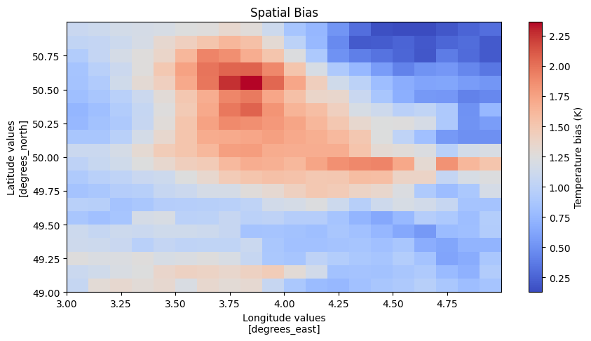
diag = vp.Model2Ref(spatial_bias, plot_spatial_bias, name="spatial_bias", description="Calculate the time averaged spatial bias between the model and the observations")
#Apply the
#Expects tas
def warming_levels(ds, ref, levels=[1.5, 2.0], rol_years=21):
#Calculate the warming levels
ref_temp = ref.tas.mean()
def calc_crossing_time(xr, wl, base, rol_years=21):
try:
rol = xr.rolling(time=rol_years*12).mean().mean(dim=['lat','lon'])
rol = rol - base
days = int(365.24*(rol_years-1)/2)
return rol.where(rol>wl, drop=True).idxmin('time').astype('datetime64[ns]').values - np.timedelta64(days,'D')
except ValueError:
return False
ds = diag.apply(dt.ensembles.cmip6.EC_Earth3.hist, dt.obs.EOBS)
ds
[9]:
<xarray.DataArray 'tas' (lat: 20, lon: 20)> Size: 2kB
dask.array<sub, shape=(20, 20), dtype=float32, chunksize=(20, 20), chunktype=numpy.ndarray>
Coordinates:
height float64 8B 2.0
* lon (lon) float64 160B 3.05 3.15 3.25 3.35 3.45 ... 4.65 4.75 4.85 4.95
* lat (lat) float64 160B 49.05 49.15 49.25 49.35 ... 50.75 50.85 50.95- lat: 20
- lon: 20
- dask.array<chunksize=(20, 20), meta=np.ndarray>
Array Chunk Bytes 1.56 kiB 1.56 kiB Shape (20, 20) (20, 20) Dask graph 1 chunks in 32 graph layers Data type float32 numpy.ndarray - height()float642.0
- units :
- m
- axis :
- Z
- positive :
- up
- long_name :
- height
- standard_name :
- height
array(2.)
- lon(lon)float643.05 3.15 3.25 ... 4.75 4.85 4.95
- units :
- degrees_east
- long_name :
- Longitude values
- axis :
- X
- standard_name :
- longitude
array([3.04986, 3.14986, 3.24986, 3.34986, 3.44986, 3.54986, 3.64986, 3.74986, 3.84986, 3.94986, 4.04986, 4.14986, 4.24986, 4.34986, 4.44986, 4.54986, 4.64986, 4.74986, 4.84986, 4.94986]) - lat(lat)float6449.05 49.15 49.25 ... 50.85 50.95
- units :
- degrees_north
- long_name :
- Latitude values
- axis :
- Y
- standard_name :
- latitude
array([49.049861, 49.149861, 49.249861, 49.349861, 49.449861, 49.549861,
       49.649861, 49.749861, 49.849861, 49.949861, 50.049861, 50.149861,
       50.249861, 50.349861, 50.449861, 50.549861, 50.649861, 50.749861,
       50.849861, 50.949861])
- lonPandasIndex
PandasIndex(Index([ 3.049860378785798, 3.149860378385746, 3.2498603779856943, 3.3498603775856424, 3.4498603771855905, 3.5498603767855386, 3.6498603763854867, 3.7498603759854348, 3.849860375585383, 3.949860375185331, 4.049860374785279, 4.149860374385227, 4.249860373985175, 4.349860373585123, 4.449860373185071, 4.5498603727850195, 4.649860372384968, 4.749860371984916, 4.849860371584864, 4.949860371184812], dtype='float64', name='lon')) - latPandasIndex
PandasIndex(Index([ 49.04986053396604,  49.14986053364869,  49.24986053333134,
          49.349860533014,  49.44986053269666,  49.54986053237931,
       49.649860532061965,  49.74986053174462,  49.84986053142728,
       49.949860531109934, 50.049860530792586, 50.149860530475245,
         50.2498605301579, 50.349860529840555,  50.44986052952321,
       50.549860529205866, 50.649860528888524, 50.749860528571176,
        50.84986052825383,  50.94986052793648],
      dtype='float64', name='lat'))
As we are using dask the resulting data needs to be computed. Note that when plotting, the data is automatically computed.
[10]:
from dask.diagnostics import ProgressBar
with ProgressBar():
    ds.compute()
[########################################] | 100% Completed | 13.04 ss
Plotting#
Finaly the diagnostic has some built in plotting functionality to visualize the results. The user can tweek the visualization or make his own starting from the resulting ds.
[11]:
f = diag.visualize(dt.ensembles.cmip6.EC_Earth3.hist, dt.obs.EOBS)
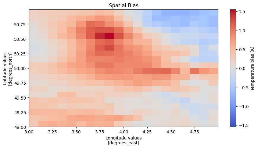
[12]:
f = diag.visualize(dt.ensembles.cmip6.EC_Earth3.ssp245, dt.obs.EOBS)